“Deep learning” describes the use of multilayer computational architectures, typically of Neural Networks, to capture a hierarchy of features embedded within the data. Some of these techniques have achieved super human performance in recent years on pattern recognition tasks. This post documents my experiments on implementing a multilayer recurrent neural network for learning musical patterns and generation. Code written in Python is hosted here.

Machine learning with Neural Networks

A typical Neural Network architecture consists of Neurons computing the weighted sum of it’s inputs and subsequently “squashing” the weighted sum with a non-linear function such as the hyperbolic tangent:

$$y_{[out_i]} = tanh\left[ \sum_{\text{neuron inputs }u^{(k)} } \left(w_{ik} u^{(k)}\right) + bias_i \right]$$

The squashing non-linearity helps the neural network to generlise. For the hyperbolic tangent function, the input can be thought of being gruoped into 3 categories, for large values of the weighted sum, no matter how large (in the practical sense), the tanh always evaluates to 1. Whereas for negative quantities, no matter how negative, the tanh function evaluates to -1. Outputs computed from weighted sum values near zero scales approximately linearly with the input. Overall, this means a large number of weighted sum result (and hence range of inputs $u^{(k)}$) are mapped to the same output value. And if the neuron is trained (with special weight configuration) to produce the same output for a group of related inputs, it possesses generalisation properties. The weights of each neuron adjusts the “preferred pattern” of the neuron. With the notation $y_{[out_i]}$ denoting the $i^{th}$ output neuron with it’s own weights $w_{i1}, w_{i2},...$ - the entire layer of neurons can be specified by the parameters $w_{ik}$ dictating how we scale the $k^{th}$ input for contributing to the $i^{th}$ output. Suppose a neuron is trained to “detect” (output firing) a large input at $u^{(1)}$ and a smaller input at $u^{(2)}$, the corresponding weight $w_{i2}$ will be large to amplify the effect of $u^{(2)}$ whereas the weight $w_{i1}$ will be small to ensure small $u^{(1)}$ inputs does not contribute to the neuron firing (i.e. output = 1). The “preferred input pattern” for a neuron to fire is termed receptive field in neural science. In computing, the receptive field of an artificial neuron can be inferrred by visualising the weights of the trained neuron, often giving us a clue on what pattern this neuron is trained to detect. In the field of machine pattern recognition, raw data is often processed to extract useful “features” before a classifier. In most cases, the selection of features determines the performance of the system. The beauty of deep network architectures is the ability of a trained network to extract useful, hierahical features of the input data to improve classification accuracy. The features picked by the network is learnt with the training data through an numerical optimisation process. In some cases this can be done without an extensive understanding of the data and without having to decide on the best set of features to be used. Of course, a thorough understanding of the data and task at hand would help to train a better network by choosing an architecture that fits the data without too much redundancies or having to resort to computationally expensive fully connected nets. (e.g. localised receptive fields are used in ConvNets for image recognition).

In our experiment of training a network to produce music, the neuron outputs represent the probability of the respective notes being played (i.e. one neuron per note). Since more than one note can be played at the same time, we don’t normalise across the output neurons as in the case of classification. Instead, we use a sigmoid function as non-linearity so the outputs are always between 0 and 1. The purpose of training is to maximise the probability of the network producing a set of desired notes $k_i$ specified in the training set together with the input examples. For this we can use a simple squared error cost:

$$C = \frac{1}{2} \sum_{i} (y_i - k_i)^2$$

so when the squared error cost is small, the network is likely to produce the desired outputs correctly. To minimise the squared error cost we differentiate the cost function w.r.t the weights of the network and update weights at each training iteration according to:

$$w_{ik} \vert_{new} = w_{ik} \vert_{old} - \text{ update rate } \frac{\partial C}{\partial w_{ik}}$$

After a number of weight updates and with an appropriately small update rate and meaningful inputs (not just random noise), the network would normally converge to a local minimum of the cost function. This is known as gradient descent, a common optimisation process for tuning model parameters to minimise a “cost”. The gradiet $\partial C / \partial w_{ij}$ can be derived using the chain rule:

$$\frac{\partial C}{\partial w_{ik}} = \frac{\partial C}{\partial y_i} \frac{\partial y_i}{\partial \omega_{ik}}$$

This way of evaluating the partial derivative of the cost function $C$ w.r.t the weights is known as back propagation. For a simple one layer feedforward network that simply computes the squashed weighted input sum, we can derive each of the partial derivative terms for weight updates for the squared error cost function:

$$\frac{\partial C}{\partial y_i} = \frac{\partial}{\partial y_i} \left[ \frac{1}{2} \sum_{i} (y_i - k_i)^2 \right] = y_i - k_i$$

thus the partial derivative (“error”) at each of the $0,1,..i,...$ output neurons is computed by the difference in network computed probability $y_i$ (which is simply the signoid outputs) and the example probability $k_i$ (which is either 1 or 0) given the sqaured error as a cost function. The cost derivative $\partial C / \partial \omega_{ij}$w.r.t. the weight $\omega_{ij}$ can be computed via the chain rule with $\partial C / \partial \omega_{ij} = \left[\partial C / \partial y_i\right] \left[\partial y_i / \partial \omega_{ij}\right]$. Using a simple single layer network with sigmoid output function as an example, $\partial y_i / \partial \omega_{ij}$ is:

$$\frac{\partial y_i}{\partial \omega_{ij}} = sig'\left[ \sum_{\text{neuron inputs }u^{(k)} } \left(w_{ik} u^{(k)}\right) + bias_i \right]u^{(k)}$$

with $sig'$ denoting the derivative of the sigmoid. This partial derivative of the loss function can also be averaged over a number of training examples. i.e. evaluating

$$\frac{1}{N} \sum_{\text{training e.g.}} \frac{\partial C\vert _{e.g.}}{\partial w_{ik}}$$

This process is known as mini batch training and can speed up convergence significantly.

An alternative cost function is to use the cross-entropy cost function, which measues the difference between a target distribution $p(x)$ and the estimated distribution $q(x)$ of a random variable $x$:

$$-\sum_{x}p(x)log(q(x))$$

Given that the probability of note $i$ to be played is simply the output $y_i \in [0,1]$ of the $i^{th}$ neuron, and assuming the target probability provided by training data is still $k_i \in \{0,1\}$, we can compute the cross entropy loss at the output as:

$$\frac{\partial C_\text{x-En}}{\partial y_i} = -\frac{\partial}{\partial y_i} \left[ k_i log(y_i) + (1-k_i) log(1-y_i) \right] = -\frac{k_i}{y_i} + \frac{1-k_i}{1-y_i}$$

In our music generation experiment, both cost functions were used for comparison.

Recurrent Networks and LSTM

The feedforward network described above takes the input layer and performs nonlinear transformation to produce the output. Recurrent Networks are Neural Networks that compute its outputs not just with the network input but also with the previous network states or outputs. This memorising capability allows recurrent networks to handle many interesting tasks including music generation as we’ve experimented here. A typical recurrent network computes the time varying output $y(t)_i$ of the $i^{th}$ neuron according to:

$$y(t)_i = tanh\left[ \sum_{states x^{(k)}_t} \omega^{out}_{ik}x^{(k)}_t \right] \text{, with}$$ $$x^{(i)}_{t} = tanh \left[ \sum_{k^{th}\text{ inputs }u_k } \left(w^{in}_{ik} u_t^{(k)} \right) + \sum_{\text{state at t-1: } x_{t-1}^{(k)} } \left(w^{x}_{ik} x_{t-1}^{(k)} \right) + bias_k \right]$$

The index $i$ here is used to step through the $i^{th}$ state $x_t^{(i)}$ in the same layer (assuming a single layer for now) and $u_t^{(k)}$ is the $k^{th}$ input of the layer at time $t$. The input/outputs of a recurrent network thus come in the form of time series data. Note for each time step we use the same weights and bias scaling.

So we’ve seen how error can be back propagated towards the input layers and the derivative of the cost function with respect to the parameters evaluated on a feedforward network. For recurrent networks, this is slightly more complicated. At each time step $t=[0,1,2...]$, an output $[y(0), y(1), y(2),...]$ is computed by the network whereas for the purpose of training, an example output $[k^{(1)}_t, k^{(2)}_t,...]$ is also provided at each time step. Thus at each time step there is an error/cost function we can compute accoring to $E_t(y(t),k(t))$ that we can use to calculate the parameter ($\underline{\theta}$ as weights and bias) updates by computing $\partial E_t/ \partial \theta$. The recurrent network utilises the computed states $[x^{(1)}_t, x^{(2)}_t, ...]$ at time $t$ for feeding foward in time to evaluate the next states in time $[x^{(1)}_{t+1}, x^{(2)}_{t+1}, ...]$. Each time advancement stage thus involves the same parameters $\underline{\theta}$. In other words, each parameter $\theta$ contributes to the error $E_t$ at time $t$ through $[0,1,...,t]$ steps. The derivative of the parameter w.r.t. error $E_t$ at time $t$ can be derived according to the chain rule:

$$\frac{\partial E_t}{\partial \theta} = \frac{\partial E_t}{\partial x_{t-1}} \frac{\partial x_{t-1}}{\partial \theta} + \frac{\partial E_t}{\partial x_{t-2}} \frac{\partial x_{t-2}}{\partial \theta} + ... + \frac{\partial E_t}{\partial x_{0}} \frac{\partial x_{0}}{\partial \theta} =\sum_{1\leq \tau \leq t-1}\frac{\partial E_t}{\partial x_{\tau}} \frac{\partial x_{\tau}}{\partial \theta}$$

We can expand the expression $\partial E_t / \partial x_{\tau}$ by using the chain rule again:

$$\frac{\partial E_t}{\partial \theta} = \sum_{1\leq \tau \leq t-1}\underbrace{\left[\frac{\partial E_t}{\partial x_{t-1}} \frac{\partial x_{t-1}}{\partial x_{t-2}} ... \frac{\partial x_{\tau +2}}{\partial x_{\tau +1}} \frac{\partial x_{\tau +1}}{\partial x_{\tau }}\right]}_{\partial E_t / \partial x_{\tau}} \frac{\partial x_{\tau }}{\partial \theta}$$

This is the partial derivative of the cost function evaluated at time $t$ w.r.t parameter $\theta$. The error signal at each time step contributes to the partial derivative of each parameter, thus practically we compute the “error” at the output and derive back propagation expressions for each weight parameter. This is known as Back Propagation Through Time(BPTT). We will futher illustrate this process in our three layer recurrent network.The total derivative of the total cost $E$ w.r.t parameter $\theta$ is given by the sum across all cost at times $t=0,1,2,..$:

$$\frac{dE}{d\theta} = \sum_{t=0..T} \frac{\partial E_t}{\partial \theta}$$

The gradient update for each parameter are carried out iteratively according to:

$$\theta \vert _{new} = \theta \vert _{old} - \left[\text{update rate}\right] \frac{dE}{d\theta}$$

The chain rule facilitates computing the partial derivatives for weight updates through a product function of the partial derivative terms. For the simple single layer example, everytime we back propagate in time using the partial derivative $\partial x_{\tau+1} / \partial x_{\tau}$ we multiply an extra term in the following form towards the final gradient:

$$\frac{\partial x^{(i)}_{\tau+1}}{\partial x^{(k)}_{\tau}} = tanh' \left[ \sum_{k^{th}\text{ inputs }u_k } \left(w^{in}_{ik} u_{\tau}^{(k)} \right) + \sum_{\text{state at } \tau \text{-1: } x_{\tau - 1}^{(k)} } \left(w^{x}_{ik} x_{\tau - 1}^{(k)} \right) + bias_k \right]\omega^{(x)}_{ik}$$

The derivative of the tanh function evaluates to $0 \leq tanh'(\bullet ) \leq 1$ regardless of it’s argument. For back propagation through time we can have the product of many terms. As a result, the product is likely to evaluate to a very small number, rendering the gradient contribution of errors at later time steps to approach zero. This means that the recurrent network will not have the correct updates for learning data with important temporal events separated by a long duration in time. This is known as the vanishing gradient problem in training recurrent networks as well as multilayer feedforward networks, where the error have to back propagate across a large number of layers following the chain rule and results in a large number of product terms.

The vanishing gradient is one of the main hurdles of training recurrent networks with gradient based methods as the gradient updates do not fully reflect the need to steer the cost function in the correct direction towards a local minima. This is deeply rooted into the network architecture of using activation function such as the hyperbolic tangents or sigmoids. A number of remidies have been proposed to tackle the vanishing gradient updates, one of them being the Long-Short Term Memory (LSTM) architecture, where a linear memory unit is used without a nonlinear activation function. The error propagation from the memory unit itself at a later time thus do not suffer from a vanishing gradient. The short commings of using linear units in a neural network is compensated by memory “gate” units controlling whether the linear (memory) unit is updated according to the input (input gate) and whether the output of a linear unit is propagated to the layer output (output gate), as well as controlling whether the memory unit should retain its old value (forget gate). So the “neuron” unit in a LSTM is different from those of the traditional RNNs. The general LSTM architecuture specifies gate sharing with the same gate controlling a number of linear units. A graphical description of a single “neuron” cell of the LSTM is shown below. The memory variable $c_t$ is feedback to itself without nonlinearity, hence the gradient do not “vanish” over time. The gate and output unit computation involves either a logistic function or tanh nonlinearity and in principle still suffers from a vanishing gradient when the network is trained by gradient based methods. Having said that, LSTMs have shown extreme effectiveness in picking up temporal events separated by a long time lag in a large number of practical scenarios.

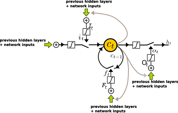
We have dropped the layer indication in the diagram such that the cell described can belong to any layer of a deep network. $h_t$ denotes the output of a hidden unit in the multilayer architecture. The overall output of the deep network is computed as the weighted sum of a number of these hidden units.

Multilayer LSTM

In a multilayer LSTM, connecting the output of each layer to the overall network output directly aids gradient back propagation for the gate parameters. The overall network architecture is illustrated below:

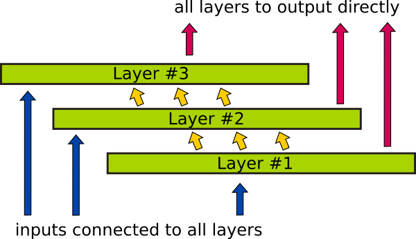
Using column vectors for the layer variables and weight matrixes while denoting element-wise multiplication by $\odot$, the forward pass in time and space of the three layer LSTM are described by:

$$\underline{i}_t^j = g_i\left[ \underline{I}_t^j \right] =g_i\left[ \boldsymbol{W}_{xi}^j \underline{x}_t + \boldsymbol{W}_{xj}^j \underline{h}_t^{j-1} + \boldsymbol{W}_{hi}^j \underline{h}_{t-1}^j + \boldsymbol{W}_{ci}^j \underline{c}_{t-1}^j + \underline{b}_i^j \right] \text{, } \\ \underline{f}_t^j = g_f\left[ \underline{F}_t^j \right] =g_f\left[ \boldsymbol{W}_{xf}^j \underline{x}_t + \boldsymbol{W}_{fj}^j \underline{h}_t^{j-1} + \boldsymbol{W}_{hf}^j \underline{h}_{t-1}^j + \boldsymbol{W}_{cf}^j \underline{c}_{t-1}^j + \underline{b}_f^j \right] \text{, } \\ \underline{c}_t^j = \underline{f}_t^j \odot \underline{c}_{t-1}^j + \underline{i}_t^j \odot tanh\left[ \underline{C}_t^j \right] \text{, }\\ \text{with }\underline{C}_t^j = \boldsymbol{W}_{xc}^j \underline{x}_t + \boldsymbol{W}_{cj}^j \underline{h}_t^{j-1} + \boldsymbol{W}_{hc}^j \underline{h}_{t-1}^j + \underline{b}_c^j \text{, } \\ \underline{o}_t^j = g_o\left[ \underline{O}_t^j \right] =g_o\left[ \boldsymbol{W}_{xo}^j \underline{x}_t + \boldsymbol{W}_{oj}^j \underline{h}_t^{j-1} + \boldsymbol{W}_{ho}^j \underline{h}_{t-1}^j + \boldsymbol{W}_{co}^j \underline{c}_{t}^j + \underline{b}_o^j \right] \text{, } \\ \underline{h}_t^j = \underline{o}_t^j \odot tanh\left[ \underline{c}_t^j \right] \text{, for layers }j=1,2,3$$

Where $\underline{x}_t$ is the network’s input vector at time $t$ and $\underline{h}_t^j$ denotes the output of each layer (sometimes called “hidden states”) at time $t$. $\boldsymbol{W}$ and $\underline{b}$ symbols denote network weight matrixes and bias vectors respectively. $g_i$, $g_f$, and $g_o$ are elementwise sigmoid functions applied to a column vector. The symbols $\underline{i}^j_t$, $\underline{f}^j_t$, and $\underline{o}^j_t$ respectively denotes the outputs at time $t$ of the $j^{th}$ layer’s input, forget, and output gates. For the convenience of calculating the cost gradients w.r.t the weights, we also define symbols $\underline{I}^j_t$, $\underline{F}^j_t$, and $\underline{O}^j_t$ as the respective weighted sumed inputs before nonlinearity is applied at the input, forget, and output gates. This is also illustrated in the LSTM cell figure above. $\underline{c}^j_t$ denotes the state of the memory unit at time $t$ and in layer $j$. The corresponding linear weighted sum is defined as $\underline{C}^j_t$. The network output $\underline{y}_t$ is computed by weighted sum of the output of all three layers, again we define a symbol $\underline{Y}_t$ as the output signal before the elementwise sigmoid $g_y$ is applied:

$$\underline{y}_t = g_y\left[ \underline{Y}_t \right] = g_y\left[ \boldsymbol{W}_{hy}^1 \underline{h}_t^1 + \boldsymbol{W}_{hy}^2 \underline{h}_t^2 + \boldsymbol{W}_{hy}^3 \underline{h}_t^3 + \underline{b}_y \right]$$

The three layers in our LSTM implementation are cascaded with output of one layer connected to the input of the next. However, since the overall network output receives contribution from all three layers directly, the three layers can be thought of a cascade and parallel hybrid.

Back propagation in time and space in LSTM

Following the chain rule, the backward error equations are derived for each $j=1,2,3$ layers:

$$\delta \underline{h}_t^j = \left[ g_y'\left(\underline{Y}_t\right) \odot \delta \underline{y}_t \right]\boldsymbol{W}_{hy}^j + \left[ g_i'\left(\underline{I}_{t+1}^j\right) \odot \delta \underline{i}_{t+1}^j \right]\boldsymbol{W}_{hi}^j + \left[ g_f'\left(\underline{F}_{t+1}^j\right) \odot \delta \underline{f}_{t+1}^j \right]\boldsymbol{W}_{hf}^j + \left[ g_o'\left(\underline{O}_{t+1}^j\right) \odot \delta \underline{o}_{t+1}^j \right]\boldsymbol{W}_{ho}^j + \left[ g_i'\left(\underline{I}_{t}^{j+1}\right) \odot \delta \underline{i}_{t}^{j+1} \right]\boldsymbol{W}_{xj}^{j+1} + \left[ g_f'\left(\underline{F}_{t}^{j+1}\right) \odot \delta \underline{f}_{t}^{j+1} \right]\boldsymbol{W}_{fj}^{j+1} + \left[ g_o'\left(\underline{O}_{t}^{j+1}\right) \odot \delta \underline{o}_{t}^{j+1} \right]\boldsymbol{W}_{oj}^{j+1} + \left[ \delta \underline{c}_{t+1}^j \odot \underline{i}_{t+1}^j \odot tanh'\left( \underline{C}_{t+1}^j \right) \right]\boldsymbol{W}_{hc}^j + \left[ \delta \underline{c}_{t}^{j+1} \odot \underline{i}_{t}^{j+1} \odot tanh'\left( \underline{C}_{t}^{j+1} \right) \right]\boldsymbol{W}_{cj}^{j+1}\\ \text{ }\\ \delta \underline{C}_t^j = \left[ \delta \underline{c}_{t}^{j} \odot \underline{i}_{t}^{j} \odot tanh'\left( \underline{C}_{t}^{j} \right) \right] \text{, with} \\ \delta \underline{c}_t^j = \left[ g_i'\left(\underline{I}_{t+1}^j\right) \odot \delta \underline{i}_{t+1}^j \right]\boldsymbol{W}_{ci}^j + \left[ g_f'\left(\underline{F}_{t+1}^j\right) \odot \delta \underline{f}_{t+1}^j \right]\boldsymbol{W}_{cf}^j + \\ \left[ g_o'\left(\underline{O}_{t+1}^j\right) \odot \delta \underline{o}_{t+1}^j \right]\boldsymbol{W}_{co}^j + \delta \underline{c}_{t+1}^j \odot \underline{f}_{t+1}^j + \delta \underline{h}_t^j \odot \underline{o}_t^j \odot tanh'\left( \underline{c}_t^j \right) \\ \text{ } \\ \delta \underline{O}_t^j = \delta \underline{o}_t^j \odot g_o'\left( \underline{O}_t^j \right) \text{, with }\delta \underline{o}_t^j = \delta \underline{h}_t^j \odot tanh\left( \underline{c}_t^j \right) \\ \delta \underline{F}_t^j = \delta \underline{f}_t^j \odot g_f'\left( \underline{F}_t^j \right) \text{, with }\delta \underline{f}_t^j = \delta \underline{c}_t^j \odot \underline{c}_{t-1}^j \\ \delta \underline{I}_t^j = \delta \underline{i}_t^j \odot g_i'\left( \underline{I}_t^j \right) \text{, with }\delta \underline{i}_t^j = \delta \underline{c}_t^j \odot tanh\left( \underline{C}_t^j \right)$$

From the error vectors, the weight gradients can be computed as the following outer products. All vectors are column vectors with row vector transposes:

$$\Delta \boldsymbol{W}_{xi}^j = \delta \underline{I}_t^j \cdot \underline{x}_t^{T} \text{; } \Delta \boldsymbol{W}_{xj}^j = \delta \underline{I}_t^j \cdot \left( \underline{h}_t^{j-1} \right)^{T} \text{; } \Delta \boldsymbol{W}_{ci}^j = \delta \underline{I}_t^j \cdot \left( \underline{c}_{t-1}^{j} \right)^{T} \\ \text{ } \Delta \boldsymbol{W}_{xf}^j = \delta \underline{F}_t^j \cdot \underline{x}_t^{T} \text{; } \Delta \boldsymbol{W}_{fj}^j = \delta \underline{F}_t^j \cdot \left( \underline{h}_t^{j-1} \right)^{T} \text{; }\\ \text{ } \Delta \boldsymbol{W}_{hf}^j = \delta \underline{F}_t^j \cdot \left( \underline{h}_{t-1}^{j} \right)^{T} \text{; } \Delta \boldsymbol{W}_{cf}^j = \delta \underline{F}_t^j \cdot \left( \underline{c}_{t-1}^{j} \right)^{T} \\ \text{ } \Delta \boldsymbol{W}_{xc}^j = \delta \underline{C}_t^j \cdot \underline{x}_t^{T} \text{; } \Delta \boldsymbol{W}_{cj}^j = \delta \underline{C}_t^j \cdot \left( \underline{h}_t^{j-1} \right)^{T} \text{; } \Delta \boldsymbol{W}_{hc}^j = \delta \underline{C}_t^j \cdot \left( \underline{h}_{t-1}^{j} \right)^{T} \\ \text{ } \Delta \boldsymbol{W}_{xo}^j = \delta \underline{O}_t^j \cdot \underline{x}_t^{T} \text{; } \Delta \boldsymbol{W}_{oj}^j = \delta \underline{O}_t^j \cdot \left( \underline{h}_t^{j-1} \right)^{T} \text{; }\\ \Delta \boldsymbol{W}_{ho}^j = \delta \underline{O}_t^j \cdot \left( \underline{h}_{t-1}^{j} \right)^{T} \text{; } \Delta \boldsymbol{W}_{co}^j = \delta \underline{O}_t^j \cdot \left( \underline{c}_{t}^{j} \right)^{T} \\ \text{ } \Delta \boldsymbol{W}_{hy}^j = \delta \underline{Y}_t \cdot \left( \underline{h}_t^{j} \right)^{T}$$

The weights and biases can then be updated by the above gradients (summed across time and averaged acrossed training examples) scaled by a small training rate.

Music generation with LSTM - Practical issues

The three layer LSTM is implemented using the Python/Theano (0.7) framework. Gradients were calculated using the equations above without relying on the symbolic differentiation of Theano. The main reason is that symbolic differentation took too long to compile with my setup (or may be there were bugs in the code…). The manually derived error terms also relied on assumptions such as $\underline{o}_t^j$ is independent of $\underline{c}_t^j$ while calculating $\partial \underline{h}_t^j / \partial \underline{c}_t^j$ from $\underline{h}_t^j = \underline{o}_t^j \odot tanh\left[ \underline{c}_t^j \right]$. Incorporating these assumptions in Theano’s symbolic differentiation is likely to speed things up but requires experimenting with “constant settings” in the gradient routine. On the other hand, implementing the equations directly using Theano tensor operators still results in good training speed even with my limited hardware setup (mobile 2.3GHz i5, no GPU). A rolling average of the gradient were used for each update (RMSprop). The three layer network in the experiment have 120 hidden units for each layer.

Both squared error and cross entropy cost functions are implemented in the code for experimentation. The network is initialised with all weights set to zero and a small gaussian noise to break the symmetry. All bias were set such that the network starts in the middle of all nonlinearities. E.g. for the logistic function, biases are initialised to $0.5\div [\text{#neurons in layer}]$ with a small gaussian noise whereas for tanh activated neurons, biases are initialised around zero with small amount of noise added. All weights and bias update rates are set to 0.01. The network is trained with the Nottingham database of folk tunes using the link from an official Theano example exploring a different RNN-RBM architecture for music generation. The network is trained by supplying midi files as mini-batches and the lenght of each tune in a mini-batch is set by the user. With this, shorter tunes are extended by repeats and longer tunes are truncated. Typically the network converges to a local minimum after few hundreds of gradient updates with update rates of 0.001. Further training without regularisation in the cost function results in over training of the network.

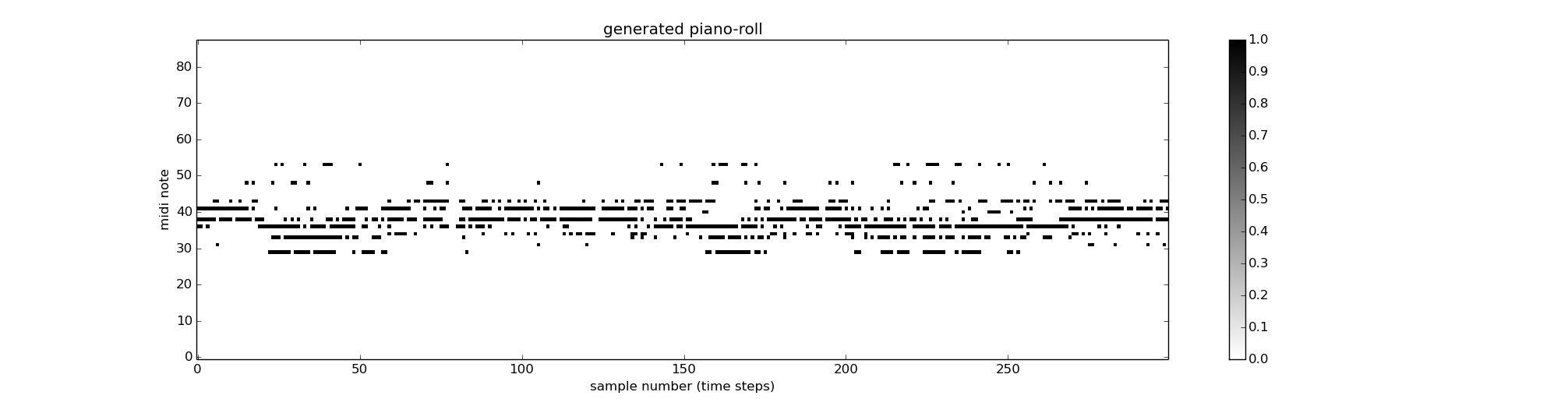
To generate music using a trained network, we first run through a few (20-100) notes from an example piece as input to the network and subsequently connect the network output as input at the next time step. Notes with probability $<0.1$ are ignored. The piano roll of a typical generated piece (mp3) with the hpps tunes in the Notthingham database with the cross entropy error cost function (300 gradient updates and 50 example points leading the generation) is shown below:

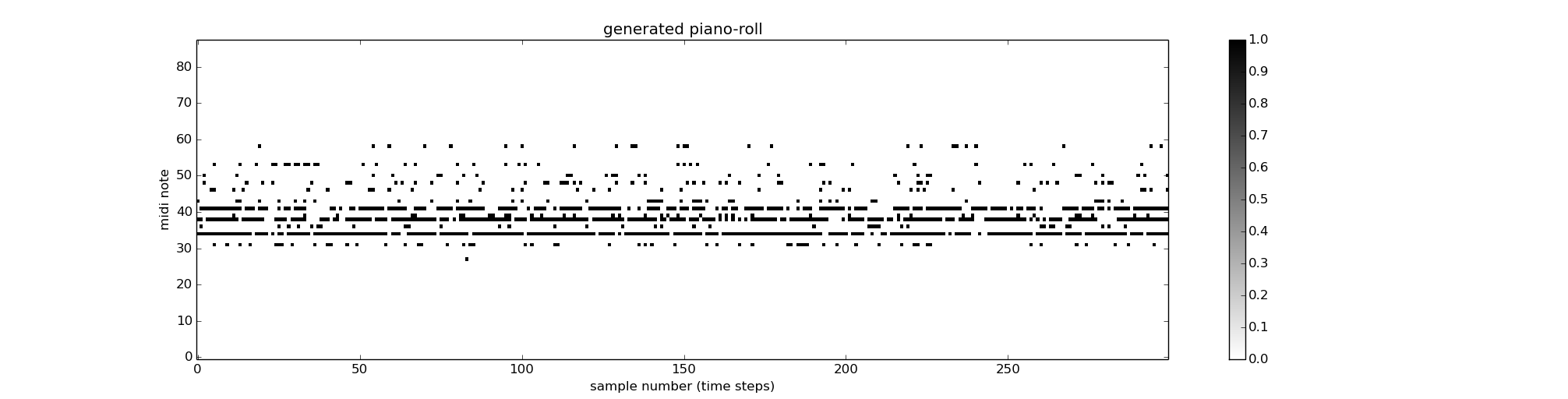
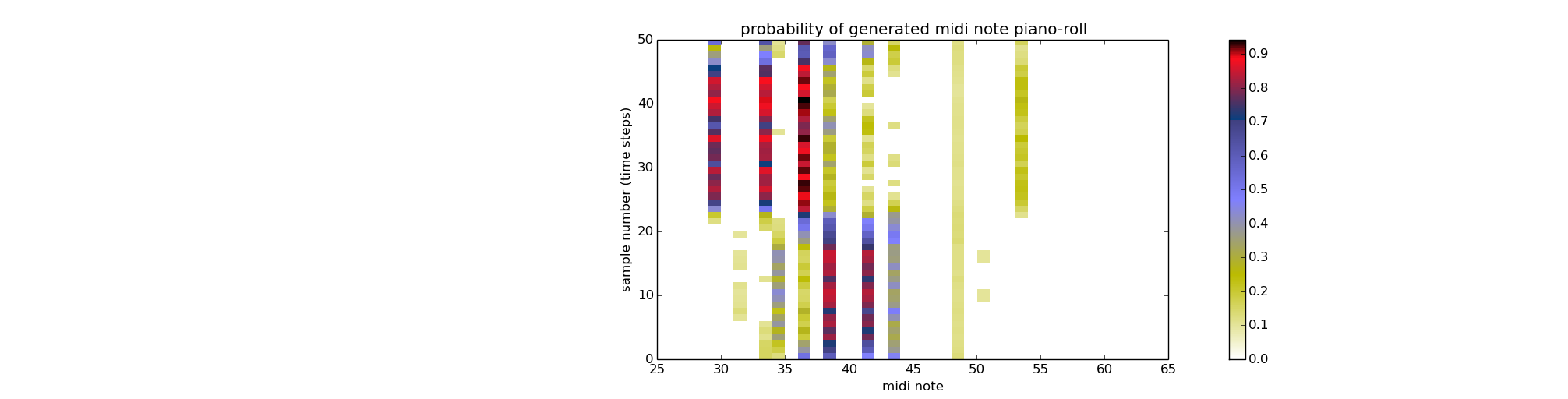
The original training data for generating the above piece consists of a large number of consecutive notes between midi notes #30 and #44. Hence the probability of generating between these notes are generally high. The typical probability of note production of the network is shown below:

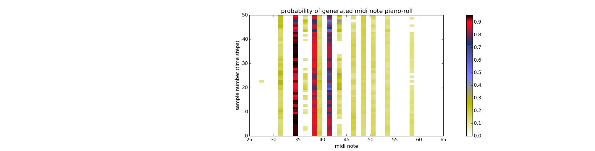
There is a clear pattern in the probability evolution with only a subset of the possible notes having a higher probability of being produced by the network. We find that with more training, the network exhibits over-training and the generation probability of each note becomes constant and resembles the average appearance probability of each note in the training set. It’s been suggested in literature that randomising the weights slightly between each gradient updates helps to prevent over-training and allow the network to pick up more subtle patterns. I am yet to experiment with this. The following shows a typical piano-roll (mp3) genearted by a network trained with the sqaure error cost function, following the same 300 gradient updates and 50 examples points leading the generation:

with corresponding probabilities for the first 50 time steps:

For more info on how to use the code seee the README on the main repository page.

References

Papers, thesis, and videos that helped me along (almost essential!) with the experiment:

1. This work is largely inspired by the official Theano example on music generation, which uses RBM and a classical RNN architecture. Also useful are the recommended Python Midi library in the link.

2. Great lecture by Andrew Ng on back propagation.

3. The Deep LSTM architecture with direct output/input connections to each layer is taken from Alex Graves “Generating Sequenes with Recurrent Neural Networks” Neural and Evolutionary Computing

4. Chapter 2 of Alex Graves’ thesis “Supervised Sequence Labelling with Recurrent Neural Networks” presented the derivation of the back prop equations for more general cases.

5. Geoffrey Hinton’s video lecture on mini batch training, Rprop, and RMSprop.