This post documents the inner workings of a statistical model (Restricted Boltzmann Machine) for modelling the joint probability of multiple random variables (R.V.s). In many real life scanarios, getting to grips with a statistical model can often give us an upper hand. In some cases we are given some data and have to work out a statistical model for it. RBMs does exactly that for multiple R.V.s. The challenge is how do we configure an RBM, which behavior depends on its parameters, to best describe the statistics of the data. Project code written in Python can be found here

Restricted Boltzmann Machines

RBM is a way of describing a joint probability of a number of random variables (two vectors $\underline{v}$, and $\underline{h}$, say), such that the probability of a particular case ($\underline{v}=\underline{v}_0, \underline{h}=\underline{h}_0$), written as $P(\underline{v}=\underline{v}_0, \underline{h}=\underline{h}_0)$ or simply $P(\underline{v}_0,\underline{h}_0)$, is proportional to the exponential of the weighted sum of these variable instances:

$$P(\underline{v},\underline{h})=\frac{1}{Z}e^{-E(\underline{v},\underline{h})}$$

with

$$E=\sum_i\sum_j\omega_{ij}h_iv_j+\sum_jb_jv_j+\sum_ic_ih_i$$

The weighted sum of the random variables $E(\underline{v},\underline{h})$ is known as the energy function and the normalisation constant $Z$ (the “partition function”) is given by summing all the possibilities of $(\underline{v},\underline{h})$:

$Z=\sum_{\underline{v},\underline{h} \in \Omega}e^{-E(\underline{v},\underline{h})}$, with $\Omega$ being the sample space of all possible combinations of $(\underline{v}, \underline{h})$.

To compute $Z$, we thus have to evaluate $e^{-E(\underline{v},\underline{h})}$ for all possible values of $(\underline{v},\underline{h})$ and sum it. This summation becomes a multiple integral for continuous, real valued $(\underline{v},\underline{h})\in \mathbf{R}^{N+M}$. The definition of the partition function $Z$ as a sum over the sample space ensures that each probability term defined by the RBM is $<1$ and all probabilities sum up to unity (more general family of densities can be found here. The overall probability of our R.V.s $(\underline{v},\underline{h})$ for the RBM, is thus given by:

$$P(\underline{v},\underline{h}) = \frac{1}{\sum_{(\underline{v},\underline{h} \in \Omega)}e^{-E(\underline{v},\underline{h})}} e^{-E(\underline{v},\underline{h})}$$

so to find the probability of a particular $(\underline{v},\underline{h})$ pair occurring, we simply substitute the $(\underline{v},\underline{h})$ pair into the above formula. The practical difficulty is the evaluation of the partition function requiring summation across the entire sample space. The structure of the RBM (as exponential of a weighted sum) also implies that any hidden R.V. in $\underline{h}=\{h_0, h_1, ..., h_{N-1}\}$ and visible R.V.s in $\underline{v}=\{v_0, v_1, ..., v_{M-1}\}$ are independent from each other in the same group when the other group is given:

$$p(\underline{h}\vert \underline{v}) = p(h_0\vert \underline{v})p(h_1\vert \underline{v})...p(h_{N-1}\vert \underline{v}) = \prod_i p(h_i\vert \underline{v})$$ $$p(\underline{v}\vert \underline{h}) = p(v_0\vert \underline{h})p(v_1\vert \underline{h})...p(v_{M-1}\vert \underline{h}) = \prod_j p(v_j\vert \underline{h})$$

This property of RBMs simplifies the sampling process. Effectively we use these conditional probabilities to generate the hidden R.V.s from given visible R.V.s and generate visible R.V.s from the previously generated hidden R.V.s:

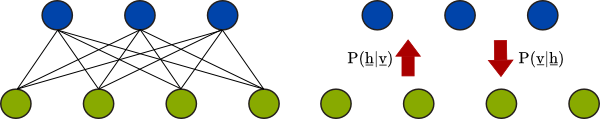
Here we illustrate a small fully connected RBM, larger RBMs are not necessarilly fully connected.

For now we treat all R.V.s in both hidden, visible layers as discrete taking 1 or 0 as values. i.e. $h_i \in \{0,1\}$, and $v_j \in \{0,1\}$ with probability defined above. Turns out in the case of binary R.V.s, writing the probability as a normalised exponential of the energy function of the random variables can represent any distribution of $(\underline{v},\underline{h})$ binary vectors. This is by tuning the parameters of the distribution $\{\omega_{ij},b_j,c_i\}$. The process of learning the distribution of a data set is thus tuning these parameters systematically such that the model approaches the statistics of the data.

In neural networks we can look at each individual neuron and characterise it with a firing probability given the states of all other R.V.s. This can be defined as the sigmoid of the weighted sum of other R.V.s:

$$\text{Prob(particular neuron firing) = sigmoid(weighted sum of other neuron states)}$$

Previously we have looked at the RBM by defining the joint probability of all R.V.s in one equation. If we extract the probability of each R.V. to be equal to unity:

$P(h_i=1\vert \text{other R.V.s fixed})$, and $P(v_j=1\vert \text{other R.V.s fixed})$

we can see the equivalent with Neural Networks. Consider the probability of a particular visible R.V. equals to 1:

$$P(v_k=1\vert \underline{v}_{\backslash k}, \underline{h})$$

,with $\underline{v}_{\backslash k}$ representing all other visible R.V. apart from $v_k$

Following conditional probability rule $P(A\vert B)P(B)=P(A,B)$, we have:

$$P(v_k=1\vert \underline{v}_{\backslash k}, \underline{h}) = \frac{P(v_k=1,\underline{v}_{\backslash k}, \underline{h})}{P(\underline{v}_{\backslash k}, \underline{h})} = \frac{P(v_k=1,\underline{v}_{\backslash k}, \underline{h})}{P(v_k=1,\underline{v}_{\backslash k}, \underline{h}) + P(v_k=0,\underline{v}_{\backslash k}, \underline{h})}$$

The last expression is derived from total probability theory. Recall that all probabilities are in the form of $e^{-E(\underline{v},\underline{h})}/Z$ so the troublesome term $Z$ actually cancels out in the fraction, leaving:

$$\frac{e^ {-\sum_{i,j\neq k}[\omega_{ij}h_iv_j] -\sum_{j\neq k}b_jv_j -\sum_ic_ih_i -b_k(1) - \sum_i\omega_{ik}h_i(1) } }{e^ {-\sum_{i,j\neq k}[\omega_{ij}h_iv_j] -\sum_{j\neq k}b_jv_j -\sum_ic_ih_i -b_k(1) - \sum_i\omega_{ik}h_i(1) } + e^ {-\sum_{i,j\neq k}[\omega_{ij}h_iv_j] -\sum_{j\neq k}b_jv_j -\sum_ic_ih_i -b_k(0) - \sum_i\omega_{ik}h_i(0) }}$$

dividing by the numerator, we have:

$$P(v_k=1\vert \underline{v}_{\backslash k},\underline{h}) = \frac{1}{1+e^{\sum_i \omega_{ik}h_i + b_k}} = sig(\sum_i \omega_{ik}h_i + b_k)$$

and similarly:

$$P(h_k=1\vert \underline{h}_{\backslash k},\underline{v}) = \frac{1}{1+e^{\sum_i \omega_{ki}v_i + c_k}} = sig(\sum_i \omega_{ki}v_i + c_k)$$

which is a sigmoid function of weighted sums of other weights! so the probability of a particular visible R.V. $v_k$ equals to one can be written as a sigmoid of weighted sums of all hidden R.V.s and a “bias” $b_k$. This is exactly like defining a neural network with the firing probability as the sigmoid of the weighted sum of states in the hidden layer. We can go from a joint distribution $P(\underline{v},\underline{h})$ defining the RBM to the individual probabilities of each R.V. reminiscent of a NN definition because the probabilities are defined as exponential functions. This allows us to simplify the probabilities with the sigmoid function, which is also based on exponentials. Despite the joint probability having the complicated partition function $Z$, the conditional probabilities are independent of $Z$. This allows us to sample from the joint probability using Gibbs sampling, which we’ll demonstrate in the code.

RBM unsupervised learning

Looking at the RBM topology again, there are no intra-layer connections (conditional probabilities). For general unsupervised learning, when we are given a set of example data $\underline{x}^{(s)}$, with unknown distribution. The task of the learning process is to model the distribution of the given data set. Often we have a model that can be used to fit the underlying distribution of the examples. To make our life easier, we have:

1. A fixed graphical structure in the model, hopefully mirroring the inter-dependencies of the data (if you know, or make an intuitive guess) e.g. RBM structure assumed. By defining a structure, one can figure out a set of analytical/computational tools to handle these specific structures (conditional probabilities)
2. some parameters in the model so we can tune to best estimate the underlying distribution of the example data set. e.g. for RBM it’s $\underline{\theta}=\{\omega_{ij},b_j,c_i\}$ in the energy function.

so how we do this with the RBM, learning the statistics from the sampled data? Tuning the parameters $\underline{\theta}=\{\omega_{ij},b_j,c_i\}$ such that it best fits the underlying distributino of the sampled data $\underline{v}^{(s)}$? The difficulty is that RBM have hidden variables $\underline{h}$, and data for this is not provided directly. Having these hidden R.V.s in the model are in fact an advantage, giving RBM the ability to capture inter-dependent (conditional) probabilities between the visible R.V.s. The input samples are generated by an unknown process, this makes it difficult to find out how well the RBM approximates the true underlying. One simple way to look at it is we tune the RBM (essentially defines a joint probability of R.V.s) parameters such that when we sample from the RBM joint distribution (i.e. using the RBM as a generative model), the probability of getting those samples back is maximum. Mathematically this is written as maximising the product (“and” relation) of probabilities of getting a particular example $\underline{v}_i^{(s)}$ given parameters $\underline{\theta}$:

$$L(\underline{\theta}\vert \underline{v}^{(s)}) = \prod_{i^{th}example} P(\underline{v}_i^{(s)}\vert \underline{\theta})$$

we label this quantity as $L(\underline{\theta}\vert \underline{v}^{(s)})$, to explicitly state that we want the parameters $\underline{\theta}$ that maximises the probability of getting the examples $\underline{v}^{(s)}$. The probability $P(\underline{v}_i^{(s)}\vert \underline{\theta})$ of getting the ith example vector $\underline{v}_i^{(s)}$ can also be written as a product of probabilities of individual elements in the ith example vector $\underline{v}_i^{(s)} = \{v_i^{(s)}(0), v_i^{(s)}(2), ... v_i^{(s)}(M-1)\}$

i.e. $P(\underline{v}_i^{(s)} \vert \underline{\theta}) = P(v_i^{(s)}(0)\vert \underline{\theta}) P(v_i^{(s)}(2) \vert \underline{\theta}) ... P(v_i^{(s)}(M-1) \vert \underline{\theta})$

to write this as a sum of terms, we take the natural logarithm:

$$ln(L(\underline{\theta} \vert \underline{v}^{(s)})) = ln(\prod_{i^{th}example} P(\underline{v}_i^{(s)} \vert \underline{\theta})) = \sum_{i^{th}example}ln(P(\underline{v}_i^{(s)} \vert \underline{\theta}))$$

This way to maximising the probability of getting the training inputs when we run our model is like minimising the “distance” between our model $P(\underline{v},\underline{h})$, and the unknown input distribution $q(\underline{v})$, say, is known as the maximum-likelihood estimation.

One way of formally measuring the difference between the example distribution $q(\underline{v})$ and our model distribution $P(\underline{v}, \underline{h})$ (strictly speaking this should be written as $P(\underline{v})=\sum_{\underline{h}}P(\underline{v},\underline{h})$ but we include the hidden vectors as they’re part of the RBM model) is the Kullback-Leibler divergence (KL-divergence):

$$KL(q||p) = \sum_{x \in \Omega}q(\underline{x})ln\frac{q(\underline{x})}{p(\underline{x})} = \sum_{x \in \Omega}q(\underline{x})ln{\left[q(\underline{x})\right]} - \sum_{x \in \Omega}q(\underline{x})ln{\left[p(\underline{x})\right]}$$

The first term is the example distribution entropy, which is fixed for a target distribution. The second term involves our model distribution $P(\underline{x})$, or $P(\underline{v})=\sum_{\underline{h}}P(\underline{v},\underline{h})$ in the RBM case. To minimise the KL-divergence between the example and model distributions we need to minimise the first term and maximise the second term as entropy functions in the form $qln(p)$ is always $\geq 0$. So how good the model approximates the example data depends on the example distribution, as distributions with lower entropy are easier to model (as they are “less random”) and others with higher entropy are harder to fit. For our model, we need to maximise the term $\sum_{\underline{s} \in \Omega}q(\underline{x})ln(p(\underline{x}))$. This is impractical to evaluate so we maximise the probability of getting the examples instead. i.e.

$$\sum_{k^{th} example}ln[P(\underline{v}_k^{(s)} \vert \underline{\theta})]$$

if our parameters $\underline{\theta} = \{ \omega_{ij},b_j,c_i \}$ maximises this then our model is “tuned” to the examples with “maximum-likelihood estimation” and achieved minimum KL-divergence between the example distribution and the model distribution. Now let’s look at the probability of running the model and generating the example vectors in detail:

$$ln(P(\underline{v}^{(s)}\vert \underline{\theta})) = ln\left[\frac{\sum_{\underline{h}}e^{-E(\underline{v}^{(s)}, \underline{h})}}{Z}\right] = ln\left[{\sum_{\underline{h}\in \Omega_h}e^{-E(\underline{v}^{(s)}, \underline{h})}}\right] - ln\left[{\sum_{\underline{v},\underline{h} \in \Omega}e^{-E(\underline{v}, \underline{h})}}\right]$$

We obtained the above expressions by substituting the example vector $\underline{v}_k^{(s)}$ into the probability expression $P(\underline{v},\underline{h})=e^{-E(\underline{v},\underline{h})}/Z$ and summing over all outcomes of $\underline{h}$, at the same time noting the partition function $Z$ is the exponential term summed over all possible values of $(\underline{v},\underline{h})\in \Omega$. Both summations involves a lot of calculations to step through. The partition function $Z$ is not constant and needs to be re-calculated as we vary the parameters $\underline{\theta} = \{ \omega_{ij},b_j,c_i \}$ during training.

So we want to tune the parameters $\underline{\theta} = {\omega_{ij},b_i,c_j}$ to maximise the log probability of examples appearing from the model. The log probability is maximised when it’s derivative with respect to the parameters is zero:

$$\frac{\partial ln(P(\underline{v}^{(s)}\vert \underline{\theta}))}{\partial \underline{\theta}} = \frac{\partial}{\partial \underline{\theta}} \left[ln\left({\sum_{\underline{h}\in \Omega_h}e^{-E(\underline{v}^{(s)}, \underline{h})}}\right) - ln\left({\sum_{\underline{v},\underline{h} \in \Omega}e^{-E(\underline{v}, \underline{h})}}\right)\right]$$ $$=>\frac{\partial ln(P(\underline{v}^{(s)}\vert \underline{\theta}))}{\partial \underline{\theta}} = \frac{-\sum_{\underline{h} \in \Omega_h} \left[e^{-E(\underline{v}^{(s)},\underline{h})} \frac{\partial E(\underline{v}^{(s)},\underline{h})}{\partial \underline{\theta}}\right] } { \sum_{\underline{h} \in \Omega_h} e^{-E(\underline{v}^{(s)},\underline{h})} } + \frac{\sum_{\underline{h},\underline{v} \in \Omega} \left[e^{-E(\underline{v},\underline{h})} \frac{\partial E(\underline{v},\underline{h})}{\partial \underline{\theta}}\right] } { \sum_{\underline{h},\underline{v} \in \Omega} e^{-E(\underline{v},\underline{h})} }$$

absorbing the total sum in the denominators:

$$\frac{\partial ln(P(\underline{v}^{(s)}\vert \underline{\theta}))}{\partial \underline{\theta}} = -\sum_{\underline{h} \in \Omega_h} \left[\frac{e^{-E(\underline{v}^{(s)},\underline{h})}}{ \sum_{\underline{h} \in \Omega_h} e^{-E(\underline{v}^{(s)},\underline{h})} } \frac{\partial E(\underline{v}^{(s)},\underline{h})}{\partial \underline{\theta}}\right] + \sum_{\underline{h},\underline{v} \in \Omega} \left[\frac{e^{-E(\underline{v},\underline{h})}} { \sum_{\underline{h},\underline{v} \in \Omega} e^{-E(\underline{v},\underline{h})} } \frac{\partial E(\underline{v},\underline{h})}{\partial \underline{\theta}}\right]$$

It is obvious that the coefficient of $\partial E(\underline{v},\underline{h})/\partial \underline{\theta}$ in the second summation on the RHS is the probability $P(\underline{v}, \underline{h})$. The coefficient of $\partial E(\underline{v}^{(s)},\underline{h}) / \partial \underline{\theta}$ in the first summation of the RHS can also be thought of as the probability $P(\underline{h}\vert \underline{v}^{(s)})$ (an exponential function of $\underline{h}$ and normalised by a summation over all possible $\underline{h} \in \Omega_h$.)

Thus the derivative of the log probability can now be written as:

$$\frac{\partial ln(P(\underline{v}^{(s)}\vert \underline{\theta}))}{\partial \underline{\theta}} = -\sum_{\underline{h} \in \Omega_h} \left[P(\underline{h}\vert \underline{v}^{(s)}) \frac{\partial E(\underline{v}^{(s)},\underline{h})}{\partial \underline{\theta}}\right] + \sum_{\underline{h},\underline{v} \in \Omega} \left[P(\underline{v},\underline{h}) \frac{\partial E(\underline{v},\underline{h})}{\partial \underline{\theta}}\right]$$

the respective summations are across all possible values of the corresponding R.V.s, we recognise these are expectation operations in the form of

$$<x> = \sum_{x\in \Omega}xP(x)$$

now we have:

$$\frac{\partial ln(P(\underline{v}^{(s)}\vert \underline{\theta}))}{\partial \underline{\theta}} = \left< \frac{\partial E(\underline{v},\underline{h})}{\partial \underline{\theta}}\right>_{\underline{v},\underline{h} \sim P(\underline{v},\underline{h}\vert \underline{\theta})} -\left< \frac{\partial E(\underline{v}^{(s)},\underline{h})}{\partial \underline{\theta}}\right> _{\underline{h} \sim P(\underline{v}=\underline{v}^{(s)},\underline{h}\vert \underline{\theta})}$$

We simply substitute appropriate samples of $(\underline{v}, \underline{h})$ into the expressions of $\partial E(\underline{v}, \underline{h}) / \partial \underline{\theta}$. the expressions of $\partial E(\underline{v}, \underline{h}) / \partial \underline{\theta}$ can be analytically derived as we have the energy function as a polynomial of the visible and hidden vectors and the parameters $\underline{\theta} = \{ \omega_{ij},b_j,c_i \}$ as coefficients.

With the probability distribution $P(\underline{v},\underline{h}\vert \underline{\theta})=e^{-E(\underline{v},\underline{h})}/Z$ dependent on the parameters $\underline{\theta}$.

To analytically calculate the true mean values one would need to sum (or integrate) over the entire sample space. Even for the second expression where we’re only concerned with all the possibilities of the hidden variable $\underline{h}$ this would be very tedious if not impossible to carry out. In practice we can estimate the respective means by drawing samples from the distributions $P(\underline{v},\underline{h}\vert \underline{\theta})$ and $P(\underline{v}=\underline{v}^{(s)},\underline{h}\vert \underline{\theta})$. However, since both distributions involve the partition function $Z$, which again requires a summation over the entire sample space to compute, we cannot obtain samples from the probability expressions directly. Instead we rely on Monte-Carlo simulations to generate approximate samples for approximating the mean terms. This approximation works in practice as in most cases we do not need the precise gradient to maximise the cost function. A gradient with the correct sign is sufficient for us to we make adjustments to the magnitude of the gradient to achieve better convergence.

Gradient ascent training

Specifically, Markov-Chain Monte-Carlo (MCMC) is a computational technique for generating samples from a known, but complicated distribution. Let’s say this distribution is $P(\underline{x})$, with $\underline{x}={x_1, x_2,...,x_n}$ being a vector of R.V.s. By taking arbitrary initial values of the R.V.s., we write them as ${x_1(0), x_2(0), ..., x_n(0)}$ and suppose we can draw a sample $x_1(1)$ from the distribution $P(x_1\vert x_2(0), x_3(0),...,x_n(0))$, and subsequently draw samples from the probability $P(x_j(k)\vert x_1(k-1), ...,x_{j-1}(k-1), ,x_{j+1}(k-1),... \text{excluding } x_j)$. If we are able to continue this process of drawing samples from the conditional probabilities $P(x_j,\vert \underline{x}_{\backslash j})$, then according to the law of large numbers, eventually the samples drawn $\underline{x}(k)$ will resemble samples drawn from $P(\underline{x})$ despite all we did was drawing samples from the conditional probabilities. This will happen regardless of the initial values $\underline{x}(0)$. Recall that generating samples from the RBM probability $P(\underline{v},\underline{h}) = e^{-E(\underline{v},\underline{h})} / Z$ directly is problematic because of the complicated partition function $Z$ but the conditional probabilities $P(v_k\vert \underline{v}_{\backslash k}, \underline{h})$ and $P(h_k\vert \underline{h}_{\backslash k}, \underline{v})$ are readily available as simple expressions. We can start with an arbitrary visible R.V. set $\underline{v}(0)$ and generate hidden R.V.s according to $P(h_k\vert \underline{h}_{\backslash k}, \underline{v})$ the newly generated hidden R.V.s are then used to generate a new set of visible R.V.s according to $P(v_k\vert \underline{v}_{\backslash k}, \underline{h})$. This process is repeated and as we go through more iterations, the generated samples will resemble more of the samples generated by the RBM probability $P(\underline{v}, \underline{h})$. So despite we cannot evaluate the joint probability $P(\underline{v}, \underline{h})$, the process of MCMC simulation allows us to draw approximate samples from the RBM. We use these MCMC samples in the gradient equation to approximate the expectation and hence the gradient. We then update the parameters according to the gradient as to maximise the probability of obtaining the training examples with our model. i.e.

$$\frac{\partial ln(P(\underline{v}^{(s)}\vert \underline{\theta}))}{\partial \underline{\theta}} = \left< \frac{\partial E(\underline{v},\underline{h})}{\partial \underline{\theta}}\right>_{\underline{v},\underline{h} \sim MCMC} -\left< \frac{\partial E(\underline{v}^{(s)},\underline{h})}{\partial \underline{\theta}}\right> _{\underline{h} \sim MCMC}$$

and

$$\underline{\theta}\vert _{new} = \underline{\theta}\vert _{old} + \text{[update rate] } \frac{\partial ln(P(\underline{v}^{(s)}\vert \underline{\theta}))}{\partial \underline{\theta}}$$

Practically the update rate is a small number (e.g. 0.001). This process of updating the parameters $\underline{\theta}$ by a small amount proportional to the gradient at each iteration in order to maximise the probability is known as gradient ascent.

So we know the MCMC process will eventually ‘converge’ if we run enough simulation steps. i.e. the generated samples from the conditional probabilities will resemble samples generated by the joint probability. But how many simulations is enough? Theory only guarantees the simulation will converge after a large number of steps but does not allow us to predict the number of simulations required. Thankfully, the exact gradient is not required for the gradient ascent algorithm to work. A gradient estimate by running a few MCMC steps will be sufficient to guide the parameter update in the right direction. In our experiments, a running average of estimated gradients over consecutive sets of training examples seems to work better than using the gradient estimate directly. In the extreme case a single MCMC step can be carried out, exploiting the fact that the gradient involves expectation terms. These are approximated with expectations of the conditional probabilities i.e. simply substitute $(\underline{v},\underline{h})$ by $\left<\underline{v}\right>_{\underline{v} \sim P(\underline{v}\vert \underline{h})}$ and $\left<\underline{h}\right>_{\underline{h} \sim P(\underline{h}\vert \underline{v})}$. For binary R.V.s the conditional probabilities are Bernoulli probabilities with the expected value equal to the probability of drawing a $1$. These are given by the sigmoid functions described above in $P(h_k=1\vert \underline{h}_{\backslash k},\underline{v})$ and $P(v_k=1\vert \underline{v}_{\backslash k},\underline{h})$

The trick of using the analytically calculated mean values without carrying out sampling are known as mean field updates. Whereas the process of estimating the gradient with truncated MCMC steps is known as contrastive divergence. This was one of the main breakthroughs that allowed training RBMs of usable size possible.

Modeling joint probability of real valued R.V.s

The Restricted Boltzmann Machine can model any joint distribution of binary R.V.s. The size of the RBM required to model an arbitrary binary distribution depends on the distribution itself as well as the number of R.V.s in the example data set. Indeed, the probability maximisation derived above (maximum-likelihood) is for a general energy function $E(\underline{v},\underline{h})$. The R.V.s $\underline{v}$ and $\underline{h}$ can be binary or real. For binary R.V.s we can use the conditional probabilities derived above in the MCMC process to estimate the gradient updates. For real visible R.V.s. with binary hidden R.V.s we can use the energy function:

$$E(\underline{v},\underline{h}) = \sum_i \frac{(v_i-a_i)^2}{2\sigma_i^2} - \sum_i \sum_j \omega_{ij}h_j\frac{v_i}{\sigma_i^2} - \sum_j b_j h_j$$

just like the binary RBM, we derive the probability $P(v_k\vert \underline{v}_{\backslash k}, \underline{h})$ independent of the partition function $Z$ as:

$$P(v_k\vert \underline{v}_{\backslash k}, \underline{h}) = \frac{P(v_k,\underline{v}_{\backslash k}, \underline{h})}{P(\underline{v}_{\backslash k}, \underline{h})} = \frac{P(\underline{v}, \underline{h})}{\int{P(\underline{v},\underline{h})}dv_k}$$

writing this in terms of the energy function and using results of standard integrals:

$$=> P(v_k\vert \underline{v}_{\backslash k}, \underline{h}) = \frac{e^{-\sum_i \frac{(v_i-a_i)^2}{2\sigma_i^2} + \sum_i \sum_j \omega_{ij}h_j\frac{v_i}{\sigma_i^2} + \sum_j b_j h_j}}{e^{-\sum_{i\neq k} \frac{(v_i-a_i)^2}{2\sigma_i^2} + \sum_{i\neq k} \sum_j \omega_{ij}h_j\frac{v_i}{\sigma_i^2} + \sum_j b_j h_j} \dot \displaystyle \displaystyle \int{e^{ -\frac{(v_k-a_k)^2}{2\sigma_k^2} + \sum_j \omega_{kj}h_j\frac{v_k}{\sigma_k^2} + \sum_j b_j h_j }}dv_k}$$ $$=> P(v_k\vert \underline{v}_{\backslash k}, \underline{h}) = \frac{e^{ -\frac{(v_k-a_k)^2}{2\sigma_k^2} + \sum_j\frac{\omega_{kj}h_jv_k}{\sigma_k^2} }}{ \displaystyle \int{e^{ -\frac{(v_k-a_k)^2}{2\sigma_k^2} + \sum_j \omega_{kj}h_j\frac{v_k}{\sigma_k^2} + \sum_j b_j h_j }}dv_k } = \frac{1}{\sqrt{2\pi \sigma_k^2}} e^{ -\frac{[v_k-(a_k+\sum_j \omega_{kj}h_j)]^2}{2\sigma_k^2} }$$

this is a Gaussian distribution and we write:

$$P(v_k\vert \underline{v}_{\backslash k}, \underline{h}) = \mathcal{N}(\mu=a_k+\sum_j\omega_{kj}h_j, \sigma=\sigma_k)$$

For the probability of a hidden R.V. depending on the visible R.V.s, we have:

$$P(h_k \vert \underline{h}_{\backslash k}, \underline{v}) = \frac{P(h_k,\underline{h}_{\backslash k}, \underline{v})}{P(\underline{h}_{\backslash k}, \underline{v})} = \frac{P(\underline{h}, \underline{v})}{P(h_k=1,\underline{h}_{\backslash k}, \underline{v}) + P(h_k=0,\underline{h}_{\backslash k}, \underline{v})}$$

substituting in the energy function and evaluating the total probability of the hidden random variable:

$$P(h_k \vert \underline{h}_{\backslash k}, \underline{v}) = \frac{e^{-\sum_i \frac{(v_i-a_i)^2}{2\sigma_i^2} + \sum_i \sum_j \omega_{ij}h_j\frac{v_i}{\sigma_i^2} + \sum_j b_j h_j}} {e^{-\sum_i \frac{(v_i-a_i)^2}{2\sigma_i^2} + \sum_i \sum_{j\neq k} \omega_{ij}h_j\frac{v_i}{\sigma_i^2} + \sum_{j\neq k} b_j h_j} \left[e^{\sum_i\frac{\omega_{ik}(h_k=0)v_i}{\sigma_i^2} + b_k(h_k=0)} + e^{\sum_i\frac{\omega_{ik}(h_k=1)v_i}{\sigma_i^2} + b_k(h_k=1)} \right]}$$

which simplifies to:

$$P(h_k \vert \underline{h}_{\backslash k}, \underline{v}) = \frac{e^{\sum_i\frac{\omega_{ik}(h_k)v_i}{\sigma_i^2} + b_k(h_k)}}{ e^{\sum_i\frac{\omega_{ik}v_i}{\sigma_i^2} + b_k} + 1}$$

To evaluate the probability of $h_k = 1$ we set $h_k=1$ in the numerator on the RHS:

$$P(h_k = 1\vert \underline{h}_{\backslash k}, \underline{v}) = \frac{e^{\sum_i\frac{\omega_{ik}(h_k=1)v_i}{\sigma_i^2} + b_k(h_k)}}{ e^{\sum_i\frac{\omega_{ik}v_i}{\sigma_i^2} + b_k} + 1} =sig\left(\sum_i \omega_{ik}\frac{v_i}{\sigma_i^2} + b_k\right)$$

We now have the conditional probabilities to approximate samples from $P(\underline{v}, \underline{h})$ to estimate the means for the gradient updates.

From math to code: practical aspects

RBMs with real visible units are known to be problematic to train. I have attempted an implementation with the Python/Theano (0.7) framework, which allows fast execution on a GPU. The script is written from scratch and a few tricks were experimented with training the RBM. The aim of the experiment was to learn pixel statistics from a face image data set (MIT CBCL). To speed up execution, Amazon EC2 GPU instances with the ipython notebook environment were used for development. (I used cuda 7.0, cuda 7.5 is also available at time of writing.) The simulated RBM consists of 361 (19x19) real visible units and 256 hidden binary units. Simulating the the fully connected RBM with 361 units on a GPU helped a lot in shortening the implementation time, particularly when a number of simulations were carried out to find good learning rates and initialisation parameters. The Theano 0.7 library supports GPU with 32bit floating point numbers. The trick is to ensure all data were defined as float32. For float64 data Theano 0.7 defaults to using the CPU.

All 2400 images in the training set were used for training. All pixel data were normalised to the range $[0,1]$. 50 images per mini-batch were fed to the network at a time for each gradient update. i.e. each gradient updates were computed with the average gradient over respective approximated gradients from each example in the mini-batch.

The network was trained for 2500 epochs. 15 iterations of the Monte Carlo chain were used for each traing example. Update rates for parameters $a_i$ and $b_j$ were set to 0.001 whereas update rates for parameters $\omega_{ij}$ and $z_i$ in $e^{z_i} = \sigma_i^2$ were both set to 0.00005. Each mini-batch took less than 10 seconds to train on an EC2 instance with a GRID 520 card.

The activity of the hidden units are also “sparcified” by including an extra term in the cost function to penalise the difference between a target average firing rate $p_t$ and the actual mean firing rate $\left<p_{\underline{h}}\right>$ computed from the training examples:

$$-p_t log\left<p_{\underline{h}}\right> - (1-p_t)log(1-\left<p_{\underline{h}}\right>)$$

where the mean activation can be calculated from all examples in a mini-batch:

$$\left<p_{\underline{h}}\right> = \left< sig\left(\sum_i \omega_{ik}\frac{v_i}{\sigma_i^2} + b_k\right) \right> _{\underline{v}_{e.g.}}$$

A running gradient average RMSprop was used to smooth out the gradient updates during simulation. I found this smoothing was necessary for the training to work without other “momentum” methods. The combination of mini-batch/RMSprop also drastically improved the convergence rate and the network converges to a local minimum with a lot less iterations compared to vanilla gradient ascent.

During the simulation, the “reconstruction error” was used as a benchmark for convergence progress. The reconstruction error essentially calculates the difference between the initial samples (which are the example images) of the MC chain and the result generated by the network after a few MC samples. The reconstruction error does not measure the probability cost directly but large reconstruction errors indicates the network model is significantly different than the training data distribution. (For Binary visible units, Annealed Importance Sampling estimation can be derived and used to estimate the probability cost function directly.)

The parameters $a_i$ can be thought of as the “mean” of the model whereas the parameters $\sigma_i$ can be thought of the deviation from the mean when the RBM is used as a generative model. For image data experiments, we can visualise the parameters $a_i$ and $\sigma_i$ and they should resemble the average of the training dataset. Typical parameters $\underline{a} = \{ a_0, a_1, ... \}$ and $\underline{\sigma} = \{ \sigma_0, \sigma_1, ... \}$ after 2500 epochs are shown below:

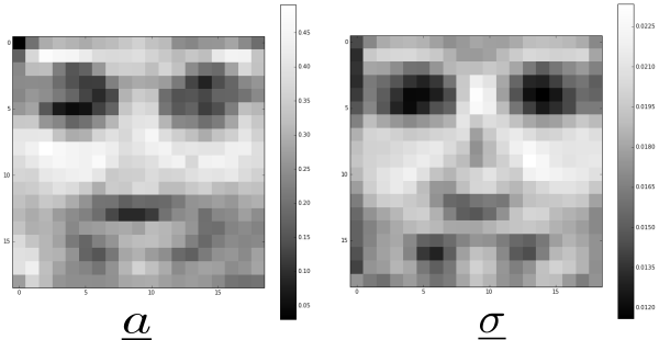
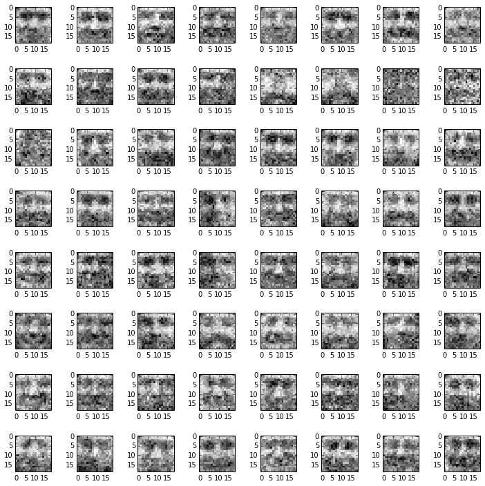
The generated images have less variety compared to the original data set. This might be due to the fact that we have a fully connected network. A multilayer deep network with localised connections for each hidden unit should work better in picking out the subtle features from the images in the training set. These samples are generated after 2500 epochs of training. Further training the network results in the generation of more homogeneous faces.

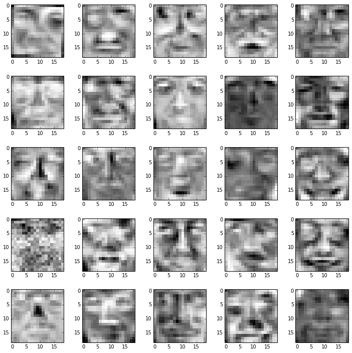
The parameters $\boldsymbol{\omega}=\{ \omega_{1,1}, \omega_{1,2},... \}$ resembles receptive fields in the sense that these are the preferred inputs to activate the hidden units. A few typical plots of $\omega_{ij}$ for fixed $i^{th}$ hidden unit and $j=\{0,1,...\}$ are shown below:

How to use the code

A brief guide to methods and parameter settings can be found with the source’s README.md

References

For RBM with real visible variables:

• “Modeling human motion using binary latent variables” by Taylor and colleagues.

• “Improved learning of Gaussian-Bernoulli Restricted Boltzmann Machines” by Cho and colleagues.

Training tricks:

• I picked up RMSprop from Geoffrey Hinton’s video lecture, also mini-batch training and Rprop.

• “A practical guide to training Restricted Boltzmann Machines” by Geoffrey Hinton provided lots of tips for training RBMs, including the sparcification of the hidden units I’ve used here.